
Directional spreading of ocean waves plays an important role in various aspects of ocean engineering, such as wave-induced loads, nonlinear wave evolution, and wave breaking. Wave following buoys, which are widely deployed across the oceans, offer the potential to measure directional wave properties. To assess the accuracy of directional spreading estimates made using buoy measurements, we compared estimates based on experimentally obtained buoy and wave gauge measurements, first presented in McAllister and van den Bremer (J Phys Oceanogr 50:399–414, 2020) Buoy and gauge measurements were recorded at the same locations and in identical sea states, allowing for a like-for-like comparison. We examine experiments with both following (unimodal in direction) and crossing (bimodal in direction) sea states. In addition to this, we use synthetic wave data to investigate the effects of wave generation and nonlinearity on spreading estimates. Our results show that while directional estimates produced using buoy measurements are reasonably accurate in following sea states, they struggle to identify distinct directional peaks in crossing sea states. We find that spreading estimates made using buoy measurements tend to underestimate the degree of directional spreading by approximately \(9-14\%\) in following sea states, which is most apparent in narrowly spread conditions.

Avoid common mistakes on your manuscript.
Waves in the oceans are three dimensional, and comprised of components that travel in different directions. Directional spreading is a measure of how wave energy for a given sea state is spread as a function of direction of propagation. Directional spreading affects wave kinematics, which in turn affects wave-induced forces on offshore structures and floating bodies (Isaacson and Sinha 1986). Extreme wave characteristics, such as nonlinearity (i.e., skewness, kurtosis) (Prevosto 1998) and wave breaking, are also critically dependent on directional spreading (Fedele 2015). These properties affect the likelihood of encountering extreme waves (Latheef and Swan 2013).
A number of devices may be used to measure ocean waves, including wave probes, wave buoys, and radars. Buoys and probes directly measure surface displacement at a single point in space. To perform conventional directional estimation, a minimum of three concurrently measured wave properties are required. In principle, wave buoys, if appropriately moored, have 6 degrees of freedom, which may be independently measured. Wave following buoys log three of these degrees of freedom, namely x, y, z displacements. Wave gauges or similar fixed Eulerian devices generally only measure vertical displacement at a single location. Thus, multiple gauges are generally required to provided directional information, whereas directional estimation may be performed using measurements from a single buoy. However, it is possible to perform indirect estimates of directional spreading using only a single Eulerian measurement by examining the magnitude of the bound harmonics (Adcock and Taylor 2009; McAllister et al. 2017).
Although buoy measurements are widely used to measure directional spreading, to our knowledge, their ability to do so has not been analysed under laboratory conditions. Benoit and Teisson (1994) compared the performance of a multi-point gauge array and a single-point gauge array which mimics the behaviour of a heave–pitch–roll buoy for directional spreading. They found that the single-point system was more effective for analysis of following sea states (unimodal in direction). Lin et al. (2020) used different quantities measured by buoys, such as displacements and velocities, to calculate spreading. They found that using velocity data resulted in the most accurate directional estimates. As buoys only measure three degrees of freedom, they may encounter issues in crossing sea states (bimodal in direction), particular when bimodality occurs over the same range of frequencies (Benoit and Teisson 1994).
In this paper, we investigate the accuracy of directional spreading estimation using wave buoy measurements through direct comparison with estimates made using an array of wave gauges in both following and crossing conditions. This paper is laid out as follows. First, we provide details of the experiments we use (Sect. 2.1), review state-of-the-art directional estimation methods (Sect. 2.2), and use synthetic data to assess our experimental setup and methods (Sect. 2.3). We use then experimental data to perform a comparison of spreading estimates made using gauge and buoy measurements in Sect. 3. We assess experiments with following and crossing directional spectra in Sects. 3.1 and 3.2, and examine the effects of mooring configuration in Sect. 3.3. Finally, we draw conclusions in Sect. 4.
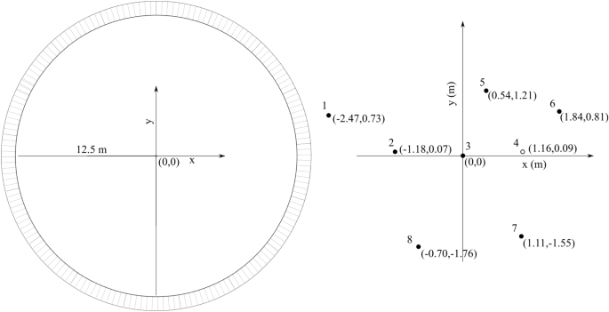
Full details of the experimental methods behind the data are given in McAllister and van den Bremer (2020). The experiments were carried out in the FloWave Ocean Energy Research Facility at the University of Edinburgh. This is a circular-wave basin surrounded by 168 absorbing wavemakers which enables the generation of waves in any direction. Figure 1 shows a schematic diagram of the wave basin, which has a 12.5 m radius and 2 m water depth.
In McAllister and van den Bremer (2020), gauge and buoy measurements were made in identical conditions at the same positions. Eight gauges and seven buoys were installed in the positions as listed in Table 1 and shown in Fig. 1. Table 2 details the targeted directional conditions of the sea states examined herein which we refer to as the input directional spreading \(\sigma _\theta \) .
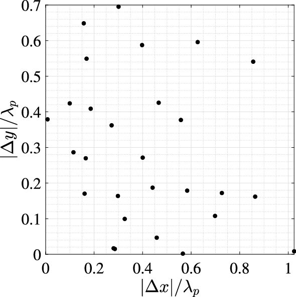
The model ‘buoys’ were plastic spheres with density half that of water, and a diameter of 0.07 m. The buoys were positioned using an auxiliary mooring; this taut mooring was highly flexible and displayed negligible effects on measured surface elevation (see McAllister and van den Bremer 2019). The mooring configuration will have an effect on lateral displacements; this is addressed in Sect. 3.3. Buoy displacements were measured using a Qualisys motion tracking system, as opposed to any on-board instrumentation. The Qualisys system uses eight infrared cameras, which simultaneously track the position of the buoys. The buoys were covered in a material that reflects infrared light. Resistive-wave gauges were used to measure surface elevation at the positions in Table 1. Figure 2 shows the separation of all possible wave gauge pairs normalised by peak wavelength \(\lambda _p\) ; this provides an indication of the range of wavelengths over which the gauge array will be effective. The wave gauge positions were chosen to provide a uniform coverage of separations over the range of relevant wavelengths, within the constraints of what was physically realisable in the wave tank.
Herein, the synthetic and experimentally generated waves were defined using a frequency spectrum \(S\left( f\right) \) based on the JONSWAP spectrum (Hasselmann et al. 1973)
typical values were taken for parameters: \(\gamma = 3.3\) , \(\sigma \left( f \le f_\mathrm
\right) = 0.07\) , and \(\sigma \left( f \>f_\mathrm
\right) = 0.09\) . For all sea states synthetic and experimental, the peak frequency \(f_\mathrm
\) is 0.6 Hz.
By measuring surface elevation at three or more points in space, or three wave quantities at a single point (i.e., x, y, z displacements for a buoy), it is possible to estimate directional spreading. The fundamental equation that relates directional spreading to observed quantities is shown below (Oltman-Shay and Guza 1984)
$$\begin
where \(\Phi _(f)\) is the cross-power spectrum of observed properties between \(m\mathrm\) and \(n\mathrm\) wave measurements, \(H_(f, \theta )\) is transfer function which converts other wave properties (i.e., velocity and acceleration) to surface elevation, \(*\) denotes the complex conjugate, S(f) is the frequency spectrum. \(x_\) , and \(y_\) represent the distances between \(m\mathrm\) and \(n\mathrm\) wave measurements. \(D(f, \theta )\) is the directional spreading function, which describes the distribution of energy as a function of direction and frequency (Benoit et al. 1997).
Estimating directional spectra accurately can be a challenge. There are infinite number of unknown parameters in Eq. (10), which makes a unique solution for the spreading function impossible when a finite number of measured wave quantities are available. To overcome this, most estimation methods use likelihood approaches to find solutions to the under-determined problem. Common methods are maximum-likelihood method (MLM) (Capon et al. 1967), iterative maximum likelihood method (IMLM) (Oltman-Shay and Guza 1984), the maximum entropy method (MEM) (Hashimoto and Kobune 1986; Lygre and Krogstad 1986), the extended maximum entropy principle (EMEP) (Hashimoto et al. 1994), and Bayesian Directional Method (BDM) (Hashimoto and Kobune 1988). See Benoit et al. (1997) and Benoit (1993) for alternative methods such as Truncated Fourier Series (Borgman 1969), Weighted truncated Fourier Series (Longuet-Higgins 1961), Eigenvector method (Marsden and Juszko 1987), and Long–Hasselmann Method (Long and Hasselmann 1979).
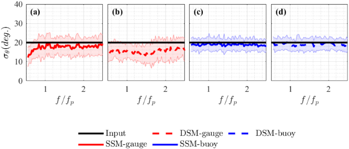
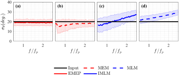
In Fig. 4, we compare directional spreading width \(\sigma _\theta \) estimated using EMEP, MEM, IMLM, and MLM methods, using 500 realisations of synthetic buoy data, which were generated using single summation method (see Sect. 2.1.1). The data were generated with a spreading width \(\sigma _\theta =20^\circ \) (see Sect. 2.2.1 for definition). The calculated quantities for each realisation were time histories of surface elevation \(\eta \) , x, and y displacements, based on linear wave theory. The directional spreading and error bounds in Fig. 4 were obtained by taking the mean and standard deviation of 500 realisations.
Directional spreading estimates made using IMLM and MLM exhibit a large offset which increases with frequency. This was also found by Young (1994) who tested synthetic pitch/roll buoy data and concluded that MLM was not capable of producing accurate estimates of directional spreading. MEM and EMEP both match the true spreading value more closely. The latter is accurate over a wider frequency range and is quicker to compute. Hence, we use EMEP in the following study. To analyse our experiments we also use an additional method of directional estimation, the Phase Time Path Difference method (PTPD) (Draycott et al. 2015). The PTPD approach can be used to estimate the direction that waves are travelling in, for experiments in which single summation wave generation is used, i.e., where only a single-wave component that travels in a single direction exists at each frequency. Draycott et al. (2015) showed that the PTPD method may be used to effectively estimate directional spectra for experimentally generated data. The PTPD method uses measured phase difference between triads of gauges to infer the direction of travel of waves at each generated frequency, and may also be used to estimate amplitude of reflected waves.
The EMEP considers errors contained in the cross spectrum when Eq. (10) is evaluated and minimises these errors to produce a unique directional spectrum. The directional spreading function is calculated using
and \(A_n(f)\) and \(B_n(f)\) \((n= 1,\ldots ,N)\) are unknown parameters which can be determined iteratively by assuming appropriate initial values. N is the order of the model chosen to minimise errors contained in the cross spectrum and Akaike’s Information Criterion (Akaike 1998). A first-order model, namely \(N= 1\) , is initially considered and higher order models are sequentially added if the models meet Akaike’s Information Criterion. Note that the order of model N should be within the half of the number of independent equations in Eq. (10).
We implement EMEP spreading estimation using the WAFO Matlab toolbox (Brodtkorb et al. 2000). We use a Hamming window without overlapping to calculate cross-spectra density. The number of Discrete Fourier Transform (DFT) points and angles for the estimated directional spectra was 2048 and 180, respectively. These parameters were chosen to optimise the resolution and stability of the output directional estimates.
Herein, when referring to spreading estimates based on buoy measurements, we present average values. This is the case in all figures unless stated otherwise. For each buoy, spreading is estimated using measured x,y, and z displacements; an average is then calculated based on the spreading estimates produced by all 7 buoys. As we produce 7 estimates of spreading, it is also possible to assess error bounds using the standard deviation of the 7 estimates. As the wave gauges each measure only a single variable namely surface elevation \(\eta \) , multiple gauges are necessary to measure spreading. To understand the error bounds of the directional estimates produced using gauge measurements, we use bootstrapping. We produced multiple estimates of spreading using all 6 gauge combinations of the 8 gauges available. Bootstrapping gives 28 estimates of spreading from which we may calculate average values and standard deviations.
For each estimated directional spreading function \(D(f,\theta )\) , we estimate the width of the spreading function \(\sigma _\theta \) at each frequency independently. For a wrapped normal distribution, the spreading width may be estimated as the standard deviation
$$\beginwhere the mean direction is calculated using
$$\beginHowever, the estimated directional distribution may not be an ideal normal distribution. Where this is the case calculating \(\sigma _\theta \) as standard deviation is sensitive to small fluctuations at large angles from the mean, and can result in disproportionately large values of \(\sigma _\theta \) . As an alternative to estimating spreading width \(\sigma _\theta \) using Eq. (13), we also calculate \(\sigma _\theta \) by fitting a normal distribution to the estimated spreading function at each frequency using a least-squares approach. Fitting a normal distribution to estimate spreading width provides a means of estimating \(\sigma _\theta \) which is less sensitive to noise than calculating the standard deviation. A comparison of these two estimation methods for calculating estimated spreading width is given in Sect. 2.3.
We apply the EMEP to time series created using linear and second-order wave theories (i.e., including second-order bound harmonics following Dean and Sharma 1981). The aim of this is to help identify any systematic errors in directional estimates that are associated with the methods and experimental setup we use. To replicate the experimental gauge array, surface elevations with the same spatial configuration were calculated. 500 realisations with input degrees of directional spreading \(\sigma _=20^\circ \) (see Table 2) were generated, and average values are taken across all of the realisations. Each realisation was 1024 s in duration and sampled at 32 Hz.
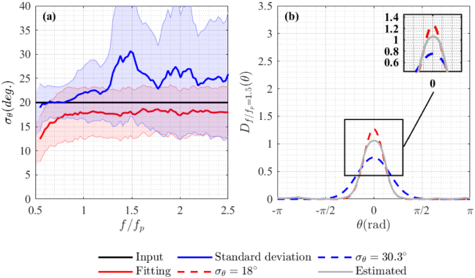
First, directional spectra were estimated using synthetic linear data. In Fig. 5a, \(\sigma _\) was calculated at each frequency using standard deviation Eq. (13) (blue line), and by fitting wrapped normal distribution to the resulting directional spreading function \(D(f_i,\theta )\) (red line). Using standard deviation to estimate \(\sigma _\theta \) results in large fluctuations with a significant increase near \(1.5f_\mathrm
\) . To illustrate why this occurs, the directional spreading function at \(1.5f_\mathrm
\) is plotted in Fig. 5b. Fitting gives a value of \(\sigma _\approx 18^\circ \) , whereas using standard deviation gives \(\sigma _\theta \approx 30.3^\circ \) . Normal distributions with spreading width \(\sigma _\theta =30.3^\circ \) and \(\sigma _\theta =18^\circ \) are shown by the blue and red dash lines, respectively. The estimated directional spreading function (grey line) is better represented by \(\sigma _=18^\circ \) (fitting) than by \(\sigma _=30.3^\circ \) Eq. (13). Spreading width calculated using standard deviation is overly sensitive to noise at large angles and fitting provides more stable estimates of spreading width. Therefore, we calculate all values of \(\sigma _\theta \) by fitting a wrapped normal distribution to estimated directional spreading functions \(D(f_i,\theta )\) herein.
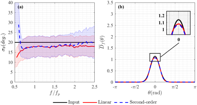
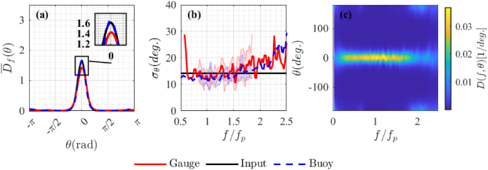
In Fig. 6, the estimated spreading width \(\sigma _\) and directional spreading function \(D(f,\theta )\) averaged over \(0.83f_\mathrm
-1.85f_\mathrm
\) , obtained for linear (red lines) and second-order (blue dashed lines) synthetic gauge data, are compared with the input degree of spreading (black lines). In Fig. 6a, estimated spreading width \(\sigma _\) is plotted as a function of normalised frequency ( \(f/f_\mathrm
\) ).
For synthetic linear data based on our experimental gauge array, the EMEP method estimates a spreading width of approximately 18.5 degrees which is stable for frequencies above \(0.75f_\mathrm
\) . This is also the case for the second-order data across the frequency range \(0.75f_\mathrm
-2f_\mathrm
\) , as frequency increases so does the estimated spreading width which also becomes less stable displaying larger error bounds. Therefore, our experimental gauge array may produce less reliable directional estimates outside the range \(0.75f_\mathrm
-2f_\mathrm
\) . For the JONSWAP spectra we examine, the amount of energy outside this range is very low (approximately \(6\%\) of the total energy).
Using the experimental data measured in McAllister and van den Bremer (2020), we examine the accuracy of directional estimates made using model buoy measurements in following (unimodal in direction) and crossing (bimodal in direction) sea states, and briefly discuss potential effects of mooring configuration.
We describe a sea state as follows if it is directionally spread about a single mean direction. In this section, several following sea states are tested (see Table 2). The same analysis procedures are applied to each experiment and average values are calculated across all of the available realisations. Each 1024 s experiment was partitioned into 16 sections with 2048 samples, which gives a frequency resolution of 0.0156 Hz and the angular resolution was defined as 2 \(^\circ \) .
Before we apply the EMEP method to the experimental data, we use the PTPD method to verify the directional conditions created during the experiments and to quantify the effects of any reflections. For experiments in which SSM wave generation is used, the PTPD method can accurately estimate the direction in which each generated wave travels and verify that the directional conditions created in the wave tank are as input. This method outputs wave direction \(\theta (f)\) at each generated frequency; to produce directional distribution \(D(f,\theta )\) , we calculate average spreading over bins of 16 discrete frequency components.
First, we investigate the sea state with input degrees of directional spreading \(\sigma _=14.14^\circ \) and steepness \(H_<\mathrm> k_<\mathrm
>/2=0.16\) . In Fig. 8, blue lines represent properties measured using buoys, and red lines represent those measured using the gauges. Both gauge and buoy measurements provide accurate results with slightly lower spreading than input values over a the frequency range \(\approx 0.7f_\mathrm
-1.8f_\mathrm
\) . On average, the values estimated using the buoy measurements are \(10\%\) lower. Estimates based on buoy measurements are accurate over slightly wider frequency range which is consistent with the results for synthetic wave data. Similar results can be also found in Benoit and Teisson (1994), which compared a single-point gauge system which approximated heave, pitch, and roll to a gauge array and found that the spreading of following sea states can be estimated more effectively by single-point system.
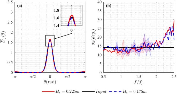
In Fig. 8, the estimated spreading width for both types of measurement is slightly smaller than the input values. For sea states that are steep, reductions in directional spreading width can occur as a result of nonlinearity (Latheef et al. 2017). The steepness of the sea states in Fig. 8 is \( H_<\mathrm> k_<\mathrm
>/2=0.16\) , which is relativity steep. The same experiments were also carried out for reduced sea state steepness, \(H_<\mathrm> k_<\mathrm
>/2=0.13\) .
In Fig. 9, we compare directional properties estimated for the two experiments carried out with input steepness \(H_<\mathrm> k_<\mathrm
>/2=0.16\) and 0.13. The estimated spreading width is slightly larger ( \(1.8\%\) on average) for the reduced steepness sea state bringing the measured values closer to the input values. Some discrepancies between input and output may still result from nonlinearity as the second sea state is still steep. The estimated spreading width increases with frequency. In Fig. 6, we showed that this may be a result of second-order bound nonlinearity. For experimental data, another reason may be that the signal-to-noise ratio becomes relatively low in both the high- and low-frequency tails of the spectrum making the waves at these frequencies appear more spread.
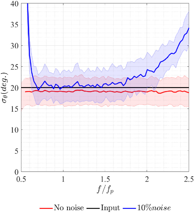
In Fig. 10, we examine the effects of noise on estimated spreading width using synthetic data. We add noise to the synthetic data using a white noise spectrum, in which rms noise amplitude was set equal to \(10\%\) of the rms amplitude of buoy displacements. For the data with noise, estimated spreading starts to deviate from expected spreading at about twice the peak frequency, whereas the estimates based on the data without noise are stable across the frequency range. Figure 8c shows directional spreading function over \(0-2.5f_\mathrm
\) . The spectrum becomes bimodal at high and low frequencies, which may make the estimated spreading disproportionally large, as well. Similar phenomenon can be found in field data (Young et al. 1995); however, in our experiments, this is most likely a result of noise, aliasing, or reflections rather than a result of the physics which drive this in the ocean. The reflection coefficients presented in Fig. 7 are approximately \(10\%\) .
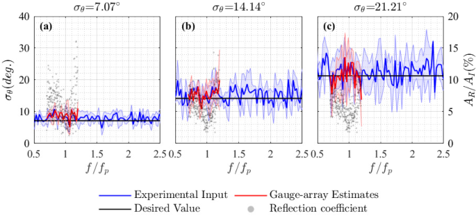
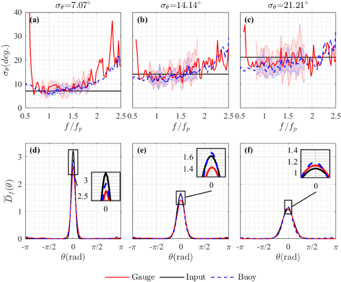
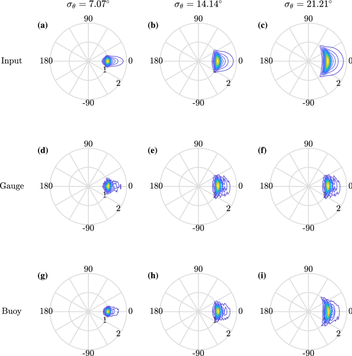
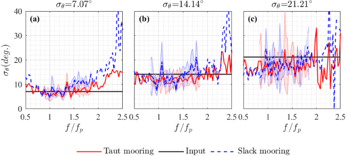
The spreading width measured using the gauge array is slightly larger than that measured by the buoys, in Fig. 8. Figure 11 shows directional estimates for all three following experiments with input degrees of directional spreading \(\sigma _=7.07^\circ \) , \(14.14^\circ \) and \(21.21^\circ \) . Red solid lines show gauge measurements and blue solid lines show buoy measurements. Transparent envelopes show error bounds (over the range \(0.83f_\mathrm
-1.85f_\mathrm
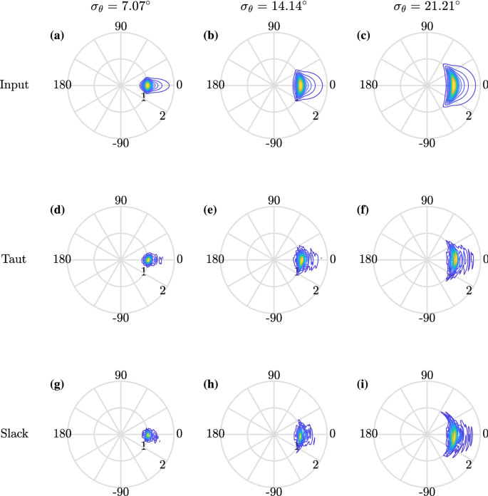
\) ). The directional spreading width estimated using buoy measurements is sightly smaller than that measured using gauges for all the cases (see Table 3). When the degree of spreading increases, the relative difference is reduced. The resulting directional spectra are illustrated as polar plots in Fig. 12.
Our observations of directional spreading show the same trend as other measured sea state parameters, such as significant wave height, skewness, and kurtosis, which differ most from gauge measurements in narrowly spread conditions (McAllister and van den Bremer 2020). In steep sea states with narrow directional spreading, increased Lagrangian transport induced by large waves may cause the apparent narrowing of the directional spectrum measured by the buoys. In Table 3, averaged values of spreading are presented. The directional spreading estimated using buoy measurements for experimentally generated following sea states is reasonably accurate, and only differs from gauge measurements by around \(10\%\) .
Crossing sea states may occur when waves generated by different weather systems combine, or during highly transient systems such as tropical storms. As only three quantities are used for directional estimates made using buoy measurements, bimodal directional distributions may present a challenge. Identifying crossing sea states is important, as they can be hazardous for seafaring vessels and potentially increase the likelihood of observing large wave crests (McAllister et al. 2019).
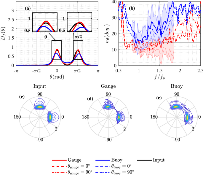
In Fig. 13, directional spectra are estimated using buoy and gauge measurements for experiments where two sea states with the same peak frequency and directional spreading \(\sigma _\theta =14.14\) cross at an angle of \(\Delta \theta =90^\circ \) . Directional estimates made using gauge measurements perform better than those made using buoy measurements, in agreement with Benoit and Teisson (1994). The spreading of two wave systems estimated using the gauges is accurate over the range from \(0.8f_\mathrm
-1.5f_\mathrm
\) , whereas the values estimated using the buoys are only accurate near the peak frequency and significantly overestimate the degree of spreading elsewhere. Estimates based on both types of measurement identify two peaks, but the definition of the peaks is worse for the buoy estimates, this is illustrated using polar plots in panel (c)–(e). The peaks of the mean directional spreading function measured by the buoys are also shifted away from each other, meaning that each perceived mean direction is incorrect and the crossing angle is overestimated (Fig. 13a).
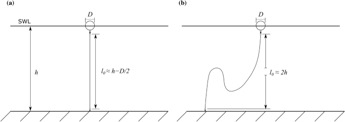
In McAllister and van den Bremer (2019), it was shown that the mooring configuration used for the experiments analysed here had no observable effect on the vertical displacement \(\eta \) . However, lateral (x, y) buoy position, which will be affected by the mooring, is important in directional estimation. In McAllister and van den Bremer (2019), additional experiments were carried out using a buoy with an alternative mooring configuration. The alternative mooring was designed to reflect more closely the type of mooring used for buoys in the ocean. The intention of this configuration, as with actual buoy moorings, is to allow for greater lateral x, y displacements. Figure 14 shows the taut and alternative ‘slack’ mooring configurations. The standard deviation of x displacement for slack mooring was 4.2 m, whereas that of original mooring was 1.12 m, indicating that the different mooring had a significant effect on lateral motion of the buoy.
In Fig. 15, directional spreading is compared for buoys with the two different moorings. Directional spreading is not significantly affected by the types of mooring near the peak frequency. However, the slack mooring appears to have an impact on the consistency of estimation, resulting in a narrower reliable frequency range (average spreading can be found in Table 3). In Fig. 16, the polar plots which correspond to the slack moored buoy are marginally less well defined than those produced using original taut mooring.
In this paper, we compare directional estimates performed using an array of gauges and individual buoys. To our knowledge, a direct comparison of gauge and buoy based estimates of spreading has not previously been carried out in the lab, where unlike the field directional spreading is defined a priori. Previous experimental studies (McAllister and van den Bremer 2019, 2020; Liu et al. 2015) have presented comparisons of measured surface elevation, extreme wave statistics and sea state parameters such as significant wave height, and peak period.
Using synthetic buoy data, we compared directional estimates produced using MEM, MLM, EMEP, and IMLM methods, and found that EMEP method provided the most stable and accurate results. This is consistent with Hashimoto et al. (1994) and Latheef et al. (2017) who also arrived at the same conclusion using synthetic wave data. Additionally, synthetic buoy data showed that a sharp increase in estimated spreading at high frequencies observed for experimental data is most likely a result of a low signal-to-noise ratio. We also demonstrate that double summation wave generation reduces the accuracy of spreading estimates made using synthetic gauge data, and show that the second-order bound nonlinearity can slightly reduce the range of frequencies over which estimates are reliable.
For following sea states based on a JONSWAP spectrum, buoy and gauge measurements produced similar estimates of directional spreading width over the range frequencies \(0.83f_\mathrm
-1.85f_\mathrm
\) for our experiments. The buoy measurements provide stable estimates of spreading over a wider range of frequencies than the wave gauge array, owing to the finite separation of the wave gauges. On average, spreading estimates based on buoy measurements were around \(10\%\) lower than those produced using gauges. At frequencies greater than around \(2f_\mathrm
\) , the estimated directional distributions became bimodal, which is most likely the combined effect of aliasing, noise, and reflections, but may also be influenced by bound nonlinearity. The same sharp increase in estimated directional spreading was also observed in the experiments performed by Latheef et al. (2017).
Both buoy and gauge-array estimates of directional spreading width were generally lower than the input spreading values. A reduction in directional spreading can occur as a result of nonlinearity for individual large wave events (Latheef et al. 2017). However, the values of spreading width measured using the PTPD method did not display a reduction in spreading, which may suggest that the underestimation we observe is a systematic issue associated with the EMEP when applied to our measurements. We also observed underestimation of spreading width when analysing synthetic linear and second-order data. Latheef et al. (2017) also observed a reduction in spreading width around the peak frequency when using six synthetic measurements of surface elevation to perform EMEP directional estimation. Our experimental observations are consistent with in situ observations made by Le Merle et al. (2021), where directional spreading estimates made using NDCB buoys (National Data Buoy Center) were shown to be on average \(3^\circ \) narrower than estimates made using scanning radar SWIM (Surface Waves Investigation and Monitoring) measurements.
In crossing sea states, buoy and gauge-array estimates of spreading were more notably different. Estimates made using the gauge array showed two distinct directional peaks and lower spreading width than the input value. Whereas, estimates made using buoy measurements significantly over predict the degree of directional spreading and struggled to identify two distinct directional peaks. The positions of the peaks were also shifted away from each other, meaning that their mean directions and perceived crossing angle were incorrect.
The two mooring configurations we examine displayed no significant differences in estimated degree of directional spreading. However, mooring dynamics may be more influential for real ocean measurements where configurations are less compliant or biofouling occurs.
Our results demonstrate that individual wave buoys are capable of producing estimates of directional spreading to reasonable degree of accuracy in simple sea sates. However, in complex crossing sea states, where multiple wave systems exist, estimates of directional spreading are significantly less accurate, and should be treated with uncertainty or validated using other measurement systems with more degrees of freedom.
This experiments used in this study were funded by the EPSRC and Wave Energy Scotland (Grant nos. 24840078 and 24841554). Mark McAllsiter was supported by the EPSRC grants EP/R007632/1 and EP/V013114/1.
This article is distributed under the terms of the Creative Commons Attribution 4.0 International License (http://creativecommons.org/licenses/by/4.0/), which permits unrestricted use, distribution, and reproduction in any medium, provided you give appropriate credit to the original author(s) and the source, provide a link to the Creative Commons license, and indicate if changes were made.